Having studied papers related to deep learning and done competitions on Kaggle, I’d like to write down my learning process. I use Python to implement most of my works and for neural network I use a powerful library Theano. Perhaps I’ll write a post about Theano some time later. Although we have a lot of Python libraries now supporting deep learning, I think Theano is one of my favourite for its flexibility and efficiency.
Note that optimization for deep nerual networks is currently a very active area of research. How to update parameters in backpropagation when using gradient descent to train a neural network is a crucial factor to its performance. I tried to compare three different techniques for parameters update in backpropagation algorithm. They are Vanilla update, Momentum update, and Nesterov Momentum. I’ll use a toy example and a multilayer perceptron (MLP) to compare those three techniques.
Before I get into the toy example, I’ll slightly introduce these three techniques. For detail, CS231n of Stanford University has more explanation. The most delicate and complete discussion can be found in [1].
Vanilla Update: It’s just a simple gradient descent algorithm. The simplest form of update is to change the parameters along the negative gradient direction.
# Vanilla update
x += - learning_rate * df
Momentum update: It’s also called classical momentum (CM). This update can be motivated from a physical perspective of the optimization problem. It is another approach that almost always enjoys better converge rates on deep networks.
# Momentum update
v = mu * v - learning_rate * df # integrate velocity
x += v # integrate position
Nesterov Momentum: The full name is Nesterov’s Accelerated Gradient or NAG. It enjoys stronger theoretical converge guarantees for convex functions and in practice it also consistently works slightly better than standard momentum.
x_ahead = x + mu * v
# evaluate df_ahead (the gradient at x_ahead instead of at x)
v = mu * v - learning_rate * df_ahead
x += v
Toy Example
The toy example is to solve a very simple problem in a numerical way and compare the results from these three techniques. For this function
,
I want to find the solution when . Obviously, the solution is . What if we use the gradient descent algorithm to find the numerical solution? Therefore, I convert this problem into a least square problem, which can be seen as
Here I implement the classical momentum technique into a function MomentumUpdate(params,learning_rate=0.01,momentum=0.9) in Theano and it can be used in all three cases.
| def MomentumUpdate(params,learning_rate=0.01,momentum=0.9):
[x, v, df] = params
v_next = momentum*v - learning_rate*df
#(variable, update expression) pairs
updates = [ (x, x + v_next ), (v, v_next) ]
return updates
|
For Vanilla Update, I only have to set the momentum to 0.0. The initial value of each variable is 0.5 and the learning rate is 0.01.
| # Declare the shared variable and initial values
x = theano.shared(np.array([0.5,0.5,0.5,0.5]).astype(np.float32))
v = theano.shared(np.zeros(4).astype(np.float32))
# Symbolic Expression
inputX = T.vector('x')
y = T.sqr(T.sum(T.sqr(inputX)))
df = T.grad(y, inputX)
updates = MomentumUpdate([x, v, df], learning_rate=0.01, momentum=0.0)
cost = theano.function(inputs=[], outputs=y, updates=updates, givens={inputX:x})
|
To do Classical Momentum, we just set the momentum to anything between 0 and 1 but 0, and have everything else remain the same. Let’s say .
| # Declare the shared variable and initial values
x = theano.shared(np.array([0.5,0.5,0.5,0.5]).astype(np.float32))
v = theano.shared(np.zeros(4).astype(np.float32))
# Symbolic Expression
inputX = T.vector('x')
y = T.sqr(T.sum(T.sqr(inputX)))
df = T.grad(y, inputX)
updates = MomentumUpdate([x, v, df], learning_rate=0.01, momentum=0.9)
cost = theano.function(inputs=[], outputs= y, updates=updates, givens={inputX:x})
|
Nesterov’s Accelerated Gradient can be implemented as below with the same learning rate and momentum as Classical Momentum.
| # Declare the shared variable and initial values
x = theano.shared(np.array([0.5,0.5,0.5,0.5]).astype(np.float32))
v = theano.shared(np.zeros(4).astype(np.float32))
# Symbolic Expression
inputX = T.vector()
x_ahead = x + momentum * v
y = T.sqr(T.sum(T.sqr(x_ahead)))
df = T.grad(y, x_ahead)
updates = MomentumUpdate([x, v, df], learning_rate=0.01, momentum=0.9)
cost = theano.function(inputs=[], outputs=y, updates=updates, givens={inputX:x})
|
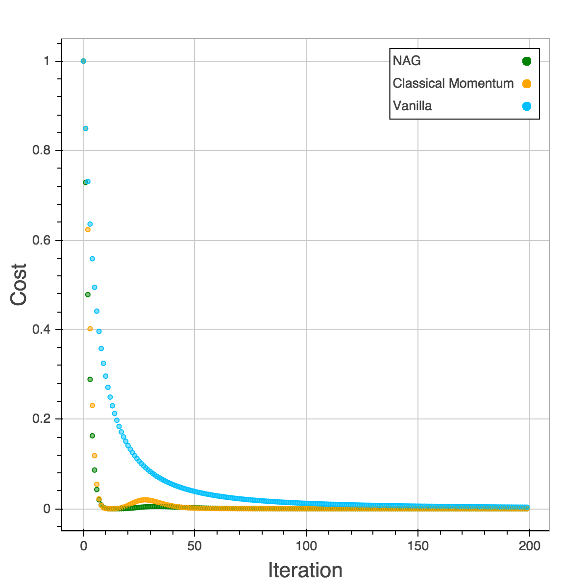
The result can be shown in below. It’s obvious that SGD is so slow that it needs almost 200 iterations to reach zero. CM and NAG are able to reach 0 within 10 iterations. We can see a small ridge appear in Classical Momentum. In this case, CM speeds up the convergence but still miss the local minimum at the first time. It’s corrected later by the momentum.
MNIST Dataset with MLP
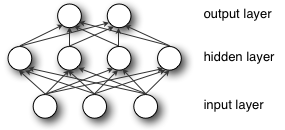
Next, I want to try a multilayer perceptron (MLP) on MNIST dataset with these three techniques. MLP is a feedforward artificial neural network model that maps sets of input data onto a set of appropriate outputs. To make things easier, I only consider one hidden layer. A single hidden layer is sufficient to make MLPs a universal approximator.
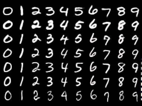
The MNIST database is a large database of handwritten digits that is commonly used for training various image processing systems. It has a training set of 60,000 examples, and a test set of 10,000 examples. Each image is 28x28 pixels.
The input numbers of neurons are , the hidden layer has 600 neurons and the output layers is a 10 classes softmax layer. I implement three techniques and the whole training and testing codes in this script. It’s slight different from the toy example with some transformation of variables. We train this MLP with mini-batch gradient descent with batch_size = 100.
| # These functions are from the script mlp.py
def sgd(cost, params, learning_rate = 0.01):
grads = T.grad(cost, params)
updates = OrderedDict()
for param, grad in zip(params, grads):
updates[param] = param - learning_rate * grad
return updates
def momentum(cost, params, learning_rate =0.01, momentum=0.9):
grads = T.grad(cost, params)
updates = OrderedDict()
for param, grad in zip(params, grads):
value = param.get_value(borrow=True)
velocity = theano.shared(np.zeros(value.shape, dtype=value.dtype),broadcastable=param.broadcastable)
updates[velocity] = momentum*velocity - learning_rate * grad
updates[param] = param + updates[velocity]
return updates
def nag(cost, params, learning_rate =0.01, momentum=0.9):
grads = T.grad(cost, params)
updates=OrderedDict()
for param, grad in zip(params, grads):
value = param.get_value(borrow=True)
velocity = theano.shared(np.zeros(value.shape, dtype=value.dtype), name="v", broadcastable=param.broadcastable)
updates[param] = param - learning_rate * grad
updates[velocity] = momentum * velocity + updates[param] - param
updates[param] = momentum * updates[velocity] + updates[param]
return updates
|
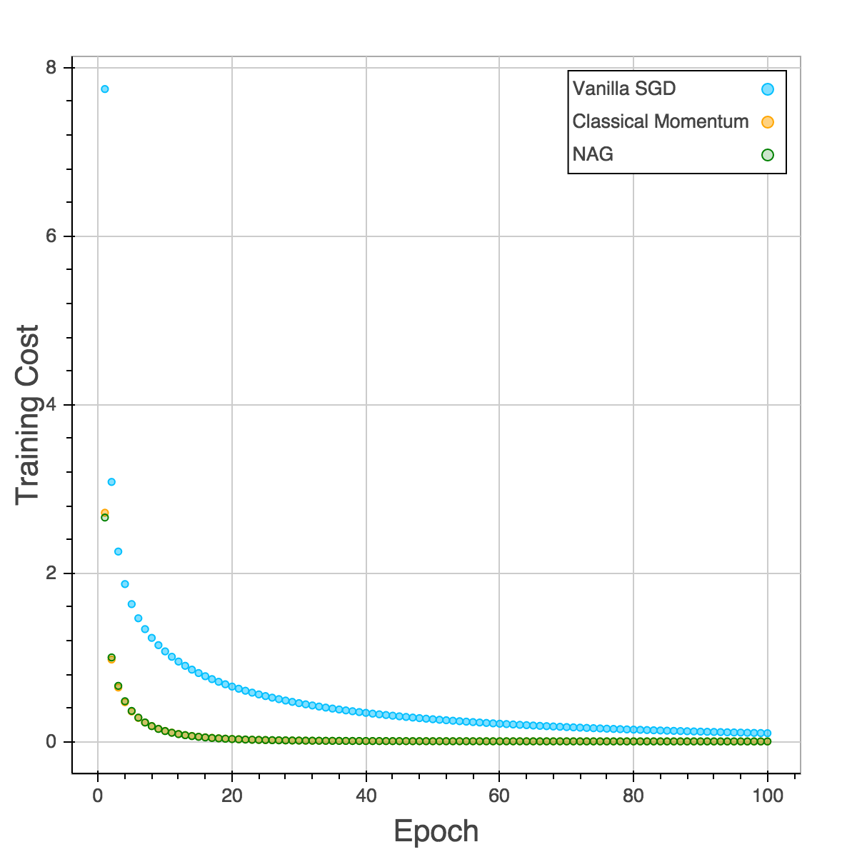
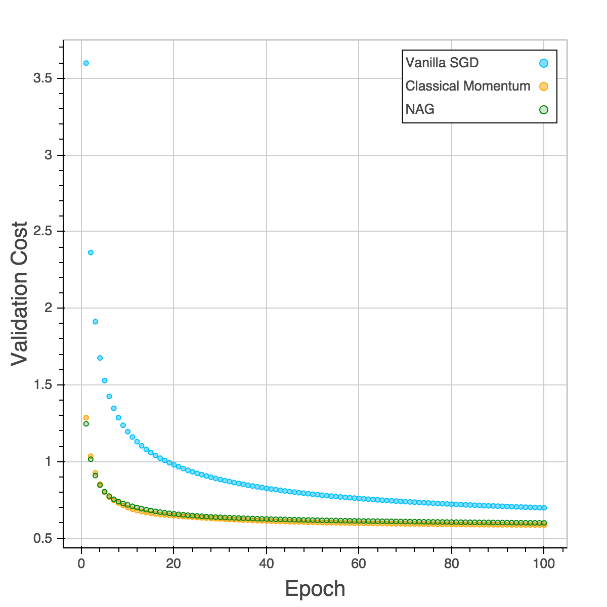
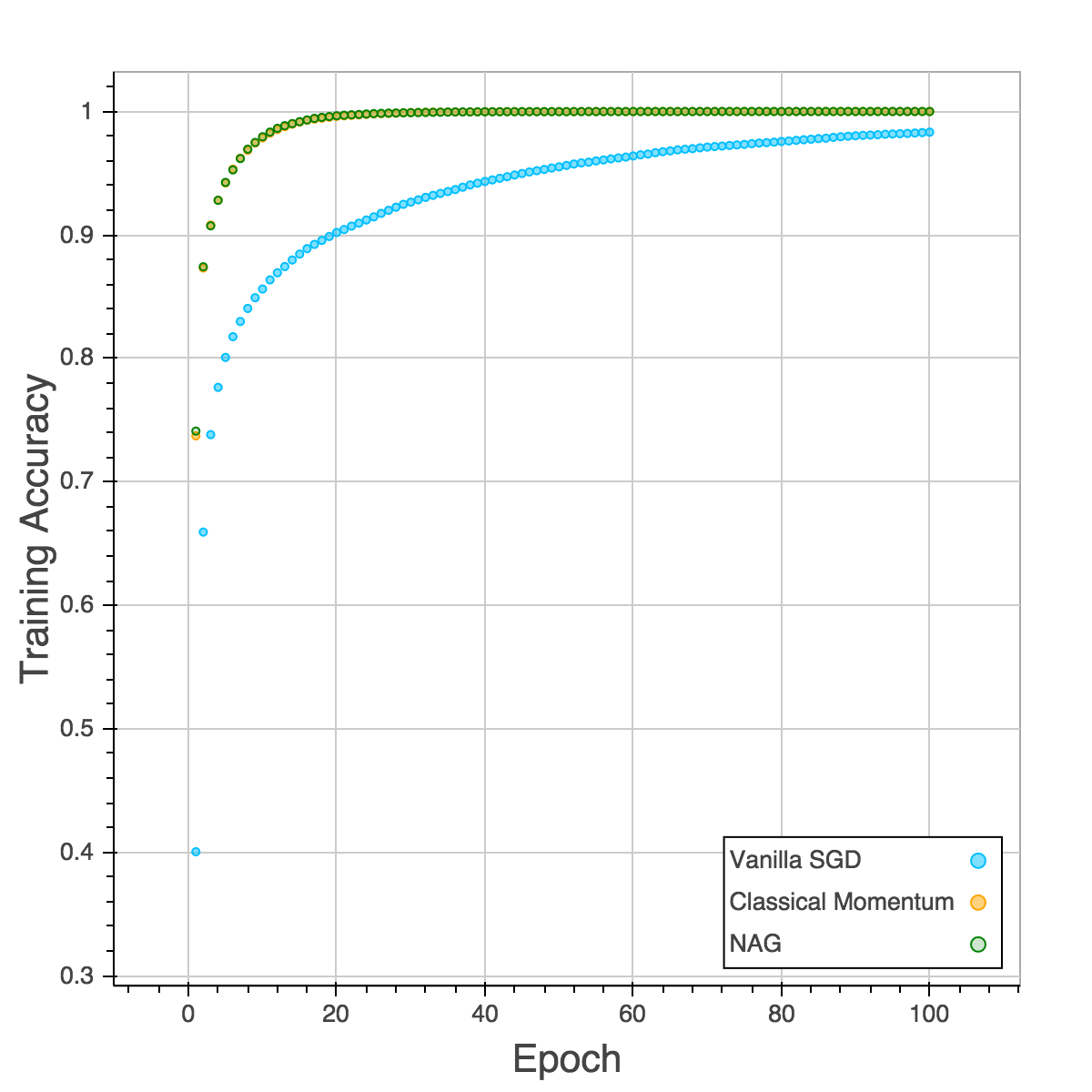
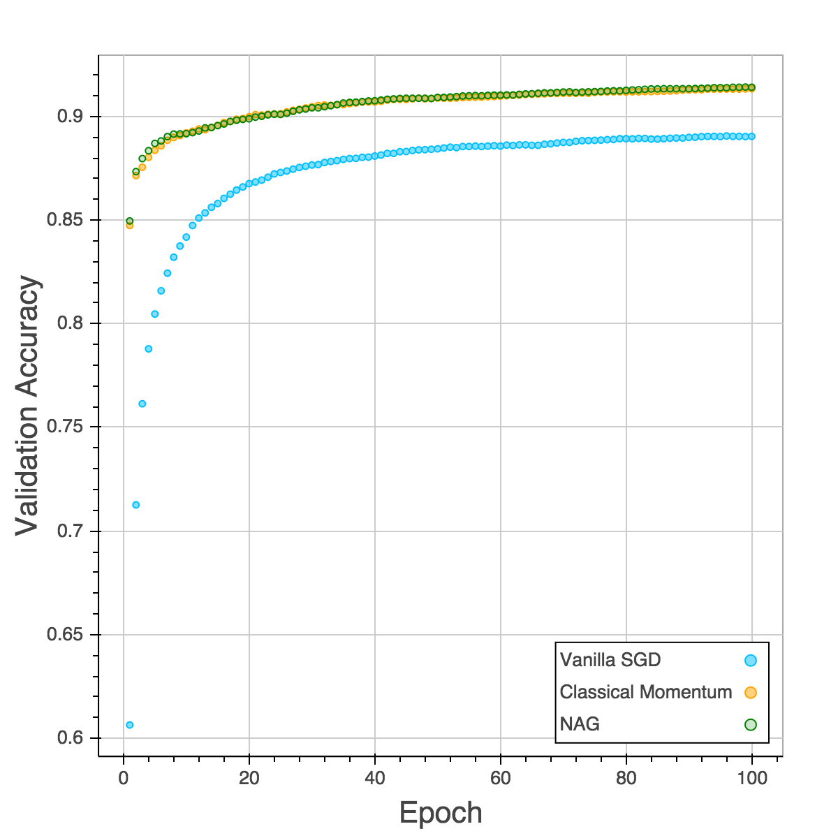
Those four plots below are training cost, validation cost, training accuracy and validation accuracy. The performances of CM and NAG are almost the same and NAG is slightly better. SGD is the slowest and easy to be trapped in local minimum as the plot of validation accuracy is shown. After training for 100 epochs, both CM and NAG reach 92% but SGD is still trapped in 89%.
Reference
Comment Section
Feel free to comment on the post.